This section is the most central function of ThinkNavi, allowing you to build and explore conceptual structure models for conceptual investigation.
Data Input
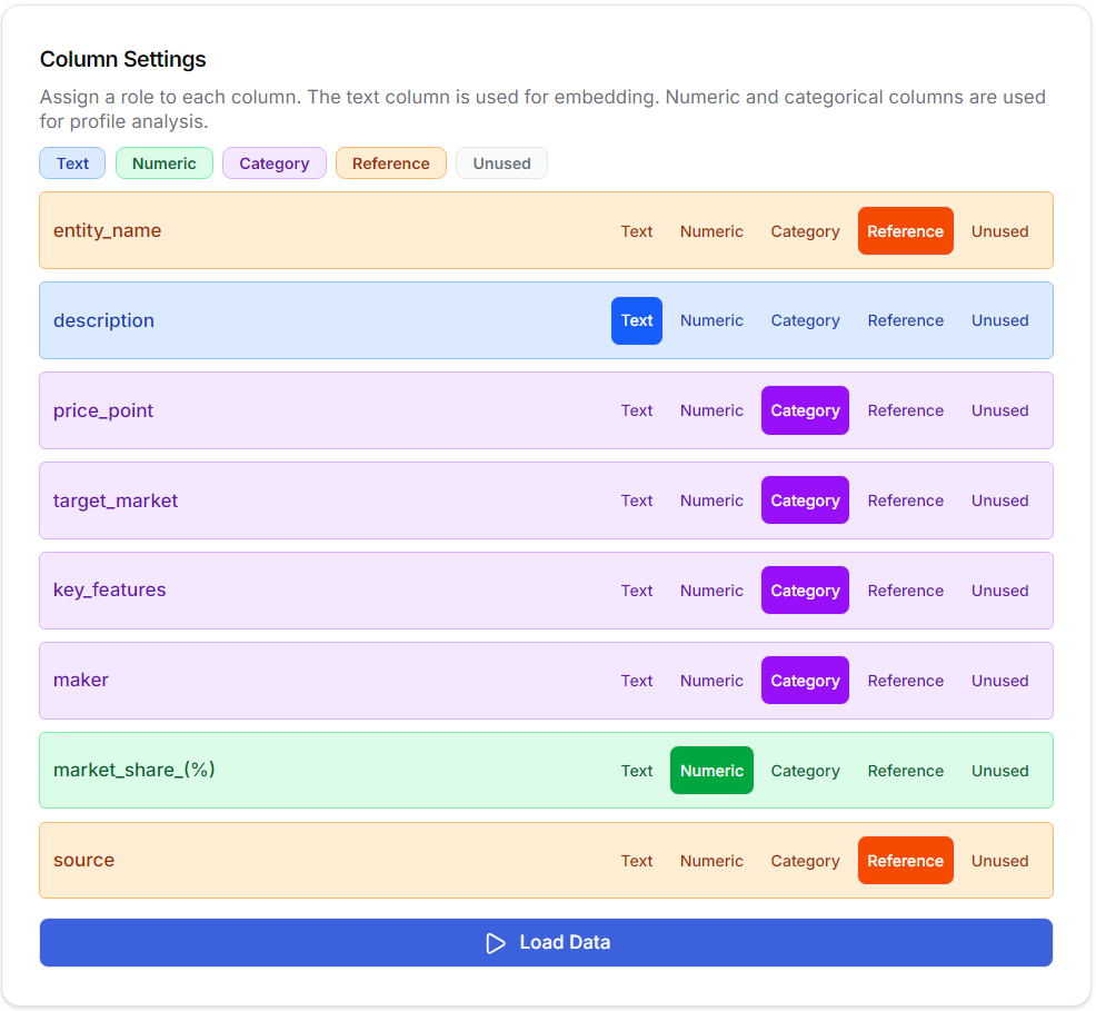
The system reads a CSV file created by Auto Research or imported from an external source, using the text columns for model creation and the numerical and categorical columns for profile analysis in the constructed model. Other columns can be used as reference columns for later reference during model exploration.
Embedding
LLM is used to obtain the text embedding vector for a specified text column. While 1536 dimensions are generally recommended, choosing a lower dimension can reduce computational cost and be used for model building trials.
Dimension Reduction
Dimensionality reduction for dimensionality interpretation is performed using UMAP (Uniform Manifold Approximation and Projection). (This is because the embedding vectors are too multidimensional for humans to interpret.) In the personal version, UMAP dimensions are used directly for model construction, but in the enterprise version, it is also possible to build the model from the embeddings. PCA+UMAP has the effect of reducing noise by running PCA before UMAP. Automatic dimensionality interpretation uses LLM to interpret and label the meaning of each dimension. Since it is necessary to understand the meaning of the dimensions in order to interpret the final model, it is especially recommended to use this function.
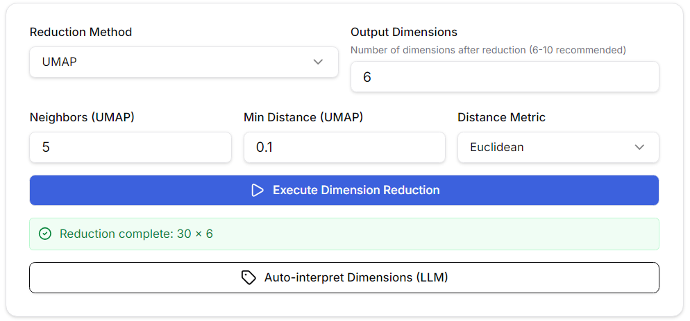
The default parameter settings for UMAP are generally fine, but in the personal version, these settings affect the node placement and clustering of the model, so adjust the number of neighbors and minimum distance as needed. A good guideline is to distribute the nodes as evenly as possible.
Feature Settings
Set the weights for each dimension. (In the enterprise version, the weights for the embedded dimensions are automatically calculated based on the correlation between each reduced dimension and the embedded dimensions.) This weighting is a key feature that defines the model’s “perspective.” Setting a weight to 0 assigns a negligible weight, meaning that dimension does not contribute to the model but is still displayed within it. Unless you have a specific purpose, it is generally best to set the weight to 1 for all dimensions.
Model Building
For model construction, you can choose between standard BGNG, fuzzy BGNG, and enhanced fuzzy BGNG. Standard BGNG is a hard assignment where each data item always corresponds to one node, while fuzzy BGNG is a soft assignment using temperature parameters, where the probability of each data item belonging to each node is calculated. Enhanced fuzzy BGNG is an extended version that appropriately maintains the distance between nodes, but usually either standard BGNG or fuzzy BGNG is sufficient.
Clustering
Clustering is performed on the nodes. The default is the Ward method (with MST constraints). This is a clustering method that uses Ward distance, but adds a rule that in hierarchical merging of clusters, clusters connected at MST edges are merged, and nodes that are not connected are not merged. As a result, clustering is obtained that follows the node topology (no cluster exclaves are created on the network).
Here too, LLM is used to automatically interpret the meaning of each cluster in the clustering results and assign labels.
Exploration
The exploration page allows you to explore the constructed model from various angles.
Network tab
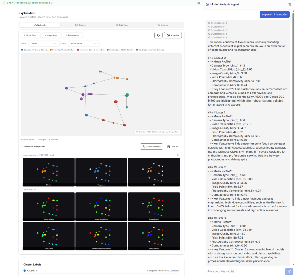
The GNG+MST model is displayed in 3D. You can switch between displaying clusters, values for each dimension, frequencies (number of records at each node), and quantization errors (errors between each node and data records). When you hover your mouse pointer over a node on the network diagram, the item name (data record) corresponding to that node will be displayed.
Profile Analysis
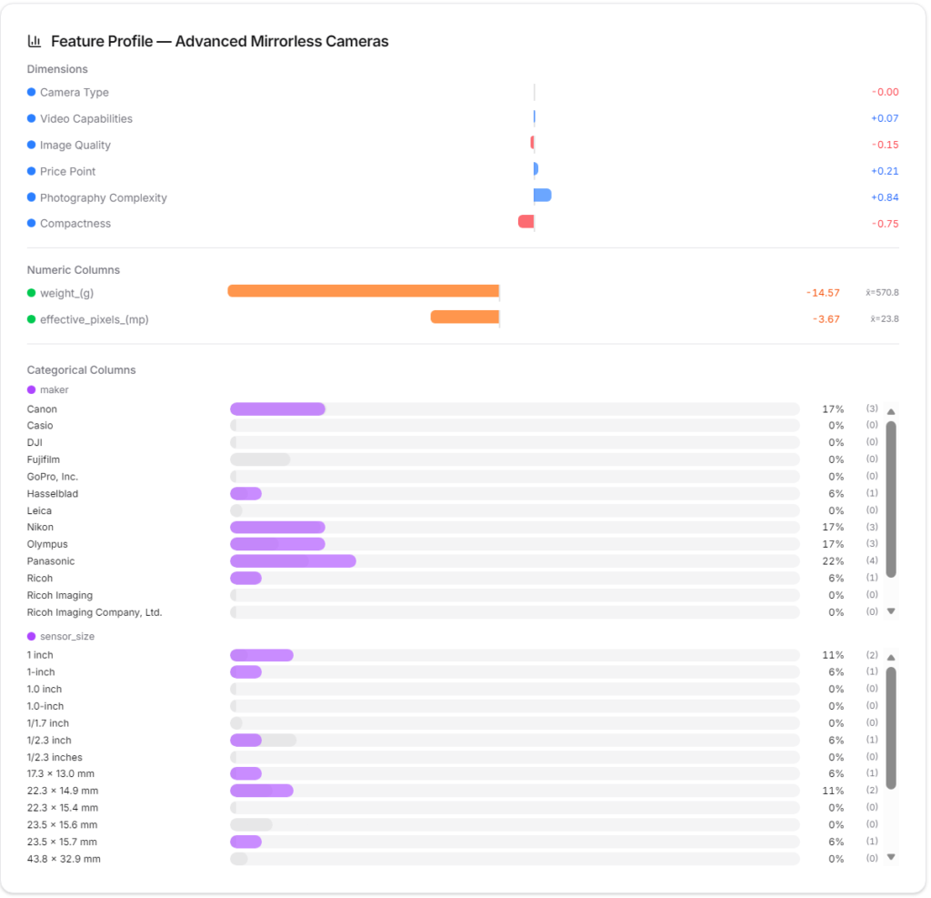
Selecting a cluster or node region will display its statistical characteristics graphically. This helps in statistically interpreting the characteristics of each part of the data space.
Cluster tab
You can examine the statistical characteristics and affiliated nodes of each cluster in detail.
Data Table tab
In the original data table, you can check the correspondence between each item (data record) and its associated node and cluster. Selecting each row will perform a profile analysis of the corresponding node.
Search tab
You can search for the corresponding item (data record) using a string and find the corresponding node.
Model Analysis Agent
ThinkNavi is equipped with an advanced model analysis AI agent. If you ask the agent “Explain this model,” it will explain the model’s overview. Or, if you ask “What is the difference between node 1 and node 21?”, it will analyze and explain in detail. Furthermore, if you ask “Starting from node 8, think of a new product concept,” it will infer a concept corresponding to the neighboring space based on the spatial relationships between the nodes.
Save / Load
Save
You can specify a project folder to save checkpoints, complete models, and shared models. Checkpoints are used to save information at intermediate stages of model building so you can continue working on them later. The complete model saves the model after it has been completed. If you select “Share,” a sharing URL will be issued. You can share the model with your colleagues by giving them this URL. Even if your colleagues do not have a ThinkNavi account, they can view a simplified version of the model in their browser. If your colleagues have a ThinkNavi account, they can view the complete model and even perform analysis using the model analysis AI agent.
Load
You can load models saved in your user project folder. You can also load shared models by entering a shared URL received from another user.
Export
You can download the model’s clustering results, all data plus dimensional information, or just the dimensional values in CSV format. You can also download the results in REFI-QDA (.qdpx), the standard data format for GTA.