

A Bayesian Network is a mathematical model that represents dependencies among events or variables using a graph and enables reasoning through probability theory. Also known as a Bayesian Belief Network (BBN), it has been widely used in artificial intelligence, fault diagnosis, medical diagnosis, risk analysis, decision support, and many other fields.
In everyday life, we constantly make decisions based on uncertain information. For example, we might reason that “If market demand increases, the probability of a new product succeeding will rise,” “If abnormal equipment behavior is detected, a particular component may have failed,” or “If business revenue declines, fixed operating costs may threaten financial stability.” However, when multiple conditions interact, it becomes difficult to evaluate these possibilities consistently through intuition alone.
Bayesian Networks provide a way to structure such judgments and calculate how the probabilities of different events change when new information becomes available. Importantly, constructing a Bayesian Network does not necessarily require large datasets or statistical learning. Experts and individual users can build models by defining network structures and probabilities based on their own knowledge and experience.
A Bayesian Network is therefore not only a technique for prediction and diagnosis but also a thinking method that helps people clarify what they know, identify their assumptions, and examine how those assumptions influence their judgments.
Basic Structure of a Bayesian Network
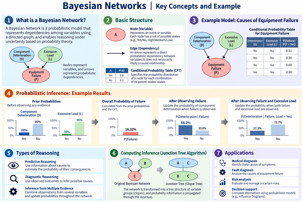
A Bayesian Network consists of three fundamental elements: nodes, edges, and Conditional Probability Tables (CPTs).
Nodes represent events or variables, such as “Market demand increases,” “Equipment fails,” or “A business succeeds.” Each node has a set of possible states, such as “Yes/No” or “High/Medium/Low.”
Edges represent direct probabilistic dependencies between variables. When an arrow connects node A to node B, the probability distribution of B is defined as depending on the state of A. However, the presence of an arrow does not by itself establish that A causally influences B.
Conditional Probability Tables (CPTs) specify the probabilities of the possible states of a node for each combination of its parent nodes’ states. Nodes without parents are assigned prior probability distributions.
For example, consider an equipment failure model in which component deterioration and excessive load influence the likelihood of equipment failure.
- Component Deterioration → Equipment Failure
- Excessive Load → Equipment Failure
In this model, the probability of equipment failure depends on the combination of component deterioration and excessive load.
Bayesian Networks are represented by Directed Acyclic Graphs (DAGs). A directed cycle, such as A → B → C → A, is not permitted. This restriction ensures that the joint probability distribution can be consistently constructed from the conditional probability distributions associated with individual nodes.
The joint probability distribution is expressed as:
P(X₁, …, Xₙ) = ∏ P(Xᵢ | Parents(Xᵢ))
This means that the joint probability distribution of all variables can be factored into a product of local conditional probability distributions. By exploiting conditional independence relationships, Bayesian Networks avoid the need to define a single enormous joint probability table directly.
Example: Diagnosing the Causes of Equipment Failure
Consider the equipment failure model described above.
Suppose the prior probability of component deterioration is 20%, while the probability of excessive load is 10%. For simplicity, assume these two variables are initially independent.
The Conditional Probability Table for equipment failure is defined as follows.
| Component Deterioration | Excessive Load | Probability of Equipment Failure |
|---|---|---|
| No | No | 1% |
| Yes | No | 50% |
| No | Yes | 60% |
| Yes | Yes | 90% |
These probabilities are hypothetical values used for illustration. In practical applications, they may be estimated from historical failure records or elicited from domain experts.
Using this network, the overall probability of equipment failure is calculated as 16.32%.
Now suppose equipment failure has actually occurred. How does this observation change the probability that a component has deteriorated?
Applying Bayes’ theorem gives:
P(Deterioration | Failure) ≈ 66.2%
The estimated probability of component deterioration increases from its prior value of 20% to approximately 66%.
Next, suppose we also discover that the equipment was operating under excessive load when the failure occurred.
The updated probability becomes:
P(Deterioration | Failure, Excessive Load) ≈ 27.3%
The probability of component deterioration decreases to approximately 27%. Because excessive load provides an alternative explanation for the failure, component deterioration is no longer considered as likely as before.
This phenomenon is known as Explaining Away. When multiple possible causes can explain an observed event, evidence supporting one cause can reduce the probability assigned to another.
Bayesian Networks can therefore perform more than straightforward predictions from causes to outcomes. They can also reason backward from observed outcomes to possible causes and update probabilities as additional evidence becomes available.
Probabilistic Inference in Bayesian Networks
Bayesian Networks support several forms of probabilistic reasoning.
Predictive Reasoning uses information about potential causes to calculate the probabilities of their consequences. For example, it can estimate how the probability of equipment failure changes when component deterioration becomes more likely.
Diagnostic Reasoning works in the opposite direction, using observed outcomes to infer possible causes. When equipment failure occurs, the network can update the probabilities of different failure mechanisms.
Inference from Multiple Sources of Evidence combines observations from several variables and updates the probability distributions throughout the network. For example, evidence such as equipment failure, abnormal vibration, and elevated temperature may progressively change the probabilities assigned to different causes.
These calculations are not limited to following the direction of the arrows. Probabilistic inference uses the dependencies encoded in the entire network, so observations may affect variables that are not directly connected.
One important computational approach is the Junction Tree Algorithm.
A Junction Tree transforms the original network into a tree-structured representation of interconnected variable groups called cliques. Probability information is propagated through this structure to calculate marginal and conditional probabilities.
When properly implemented, the algorithm performs exact probabilistic inference.
However, computational requirements can increase dramatically as network complexity grows. The difficulty depends not simply on the number of nodes but also on the size of the cliques formed during the transformation.
For large or complex models, approximate inference techniques such as sampling methods or Loopy Belief Propagation may be used.
Loopy Belief Propagation iteratively exchanges probability messages on factor graphs containing loops. It is important to distinguish these computational loops from directed causal cycles: Loopy Belief Propagation does not, by itself, allow ordinary Bayesian Networks to contain directed cycles.
Building Bayesian Networks Without Training Data
Bayesian Networks can be learned from data, including both their structures and conditional probabilities. However, from the perspective of thinking support, manually constructing a network can be equally valuable.
Consider an investment decision for a new business.
A user might identify variables such as market demand, competitive environment, technical feasibility, development costs, sales success, and business profitability.
The first task is to determine which variables directly depend on others. Rather than simply listing relevant factors, the user must consider how those factors are connected.
This process itself can deepen the understanding of the business.
The next step is to define the states of each variable and assign conditional probabilities.
For example, a user might estimate that the probability of sales success is 70% when market demand is high and competition is weak, but only 10% when demand is low and competition is strong.
Even if these estimates come from personal judgment rather than statistical data, the network can still perform mathematically consistent probability calculations.
However, the results are conditional on the assumptions encoded in the model. They do not automatically represent objectively verified probabilities.
The value of this approach lies in making judgments explicit and allowing them to be examined.
For example, if a model assigns a high probability of sales success even when technical feasibility is low, the user should examine the reasoning behind that assumption.
Similarly, if a small change in an estimated probability significantly changes the final result, the corresponding variable represents an important source of uncertainty and may deserve further investigation.
In this way, Bayesian Networks can serve as tools for transforming informal judgments into explicit, testable models, rather than simply machines for calculating answers.
Differences from Other Analytical Methods
Bayesian Networks share certain characteristics with regression analysis, decision trees, the Analytic Hierarchy Process (AHP), and causal loop diagrams. However, these methods address different kinds of problems.
Regression Analysis expresses relationships between explanatory variables and a dependent variable through mathematical equations. Interaction terms can represent situations where the effect of one variable depends on the value of another. Bayesian Networks can also represent such interactions through conditional probability distributions involving multiple parent nodes.
Decision Trees use sequences of conditional branches for classification and prediction. Bayesian Networks, by contrast, model joint probability distributions across multiple variables. This allows different variables to become the targets of inference without requiring a single predefined dependent variable.
The Analytic Hierarchy Process (AHP) is a decision-making method for determining the relative importance of evaluation criteria and ranking alternatives. Bayesian Networks instead represent uncertain events and calculate their probabilities. AHP weights and evaluation scores should not be confused with probabilities.
Causal Loop Diagrams are used in systems thinking to represent influence relationships and feedback loops. Conventional Bayesian Networks cannot directly represent directed cycles within a single time slice. However, Dynamic Bayesian Networks can model feedback processes by representing variables across successive time steps.
Each method has its own strengths and limitations. The appropriate choice depends on the structure of the problem, the information available, and the purpose of the analysis.
Limitations and Important Considerations
Although Bayesian Networks provide mathematically consistent probabilistic inference, they do not guarantee that the underlying model accurately represents reality.
If the network structure is incorrect, important dependencies may be omitted or inappropriate conditional independence assumptions may be introduced. If the Conditional Probability Tables contain inaccurate values, the results may differ substantially from actual probabilities.
Another limitation is the rapid growth of CPTs as the number of parent nodes increases.
For example, a node with five binary parents requires probabilities to be specified for 32 combinations of parent states. As networks become more complex, manually assigning probabilities can become difficult even for experienced experts.
It is also essential to distinguish probabilistic dependence from causality.
In an ordinary Bayesian Network, an arrow represents a direct dependency in the probabilistic factorization. The arrow alone does not demonstrate a causal relationship.
Observing a variable and deliberately intervening to change that variable are also different operations.
For example, the profitability of companies that naturally achieve high sales may differ from the profitability that would result if a particular intervention increased sales. Evaluating interventions requires additional causal assumptions and an appropriate causal model.
For models based on subjective probability estimates, sensitivity analysis is particularly important.
By varying the input probabilities within plausible ranges and observing how the results change, users can identify which assumptions most strongly influence their conclusions.
This helps prevent mathematically precise results from creating an unjustified impression of certainty.
Bayesian Networks and Decision-Making
A Bayesian Network can estimate the probabilities of future events or possible causes based on available evidence. However, probability estimates alone do not determine the best decision.
Suppose a new business project A has a 70% probability of success, while project B has a 40% probability.
Project A is not necessarily the better investment. Project B might generate much greater returns if successful, or it might involve substantially smaller losses if it fails.
To address such decisions, Bayesian Networks can be extended into Influence Diagrams.
An Influence Diagram adds decision nodes and utility nodes to the probabilistic structure.
Decision nodes represent actions available to the decision-maker, while utility nodes represent the value or consequences associated with different outcomes.
The model can then be used to compare the expected utilities of alternative decisions under uncertainty.
This approach is applicable to new business investments, R&D project selection, capital investment, risk mitigation, and many other decisions.
It can also be combined with AHP and other multi-criteria decision-making methods. However, the importance of evaluation criteria, probabilities of events, and utilities of outcomes must be treated as conceptually distinct quantities.
Bayesian Networks in the Age of AI
The development of Large Language Models (LLMs) has created new opportunities for constructing and using Bayesian Networks.
Traditionally, creating a model required experts to identify variables, determine dependencies, and specify probabilities.
With LLM assistance, users can describe a problem in natural language and receive suggestions for relevant variables and possible relationships.
For example, a user might enter:
“I want to analyze the likelihood of success for a new business.”
An LLM could propose variables such as market demand, development capabilities, sales channels, competitive conditions, and access to financing. It could then suggest a preliminary network structure connecting those variables.
LLMs can also help users search research reports, technical literature, and other sources for information relevant to probability estimation.
However, an LLM-generated network structure is not necessarily valid, and numerical probabilities generated by an LLM may lack empirical support.
A plausible-looking probability is not equivalent to a statistically justified estimate. Users must therefore review the assumptions, verify available evidence, and approve the resulting model.
An appropriate division of responsibilities is to use LLMs for problem interpretation, model construction assistance, and information retrieval, while assigning probability calculations to a dedicated mathematical inference engine.
This combines the flexibility of language-based reasoning with the explicit and reproducible inference provided by probabilistic models.
Bayesian Networks in ThinkNavi
ThinkNavi approaches Bayesian Networks as tools for structuring uncertain problems and examining the assumptions underlying human judgment.
ThinkNavi Free is planned to include a manually operated Bayesian Network tool that allows users to define nodes, edges, states, and Conditional Probability Tables, and then perform probabilistic inference.
The objective is to provide an accessible environment in which users can represent their own knowledge and experience without requiring large training datasets.
Planned basic capabilities include visual network editing, probability table input, posterior probability calculation based on observed evidence, comparison of different conditions, and local storage of analysis models.
In the LLM-assisted version, additional possibilities include generating candidate variables and dependencies from natural language, retrieving information relevant to probability estimation, and examining inconsistencies or weaknesses in model assumptions.
A Bayesian Network does not guarantee correct predictions. Its importance lies in making previously implicit judgments explicit, clarifying probabilistic assumptions, and showing how conclusions change when new information becomes available.
The ultimate purpose is not to delegate judgment to a computer, but to help people understand, examine, and improve their own reasoning. Bayesian Networks are among the most powerful mathematical approaches available for supporting this process.
Related Thinking Methods:
- Bayesian Inference,
- Causal Inference,
- Causal Loop Diagrams — Visualizing Feedback Structures and Understanding System Behavior
- System Dynamics — Modeling Feedback Mathematically to Understand How Systems Change Over Time
- AHP|一対比較で判断基準を整理する
- Multi-Criteria Decision Analysis (MCDA),
- Influence Diagrams
References and Further Reading
- Judea Pearl, Probabilistic Reasoning in Intelligent Systems: Networks of Plausible Inference, Morgan Kaufmann, 1988.
- Finn V. Jensen and Thomas D. Nielsen, Bayesian Networks and Decision Graphs, 2nd Edition, Springer, 2007.
- Daphne Koller and Nir Friedman, Probabilistic Graphical Models: Principles and Techniques, MIT Press, 2009.
- UC Berkeley — Bayesian Networks
- Kevin Murphy — A Brief Introduction to Graphical Models and Bayesian Networks
- pgmpy — Probabilistic Graphical Models in Python