

System Dynamics (SD) is a methodology for representing causal relationships, feedback, accumulation, and time delays within systems using mathematical models, and analyzing how those systems change over time.
Developed by Jay W. Forrester in the 1950s, System Dynamics has been applied to a wide range of fields, from production, inventory, and distribution in business organizations to urban development, economics, environmental systems, healthcare, and organizational management.
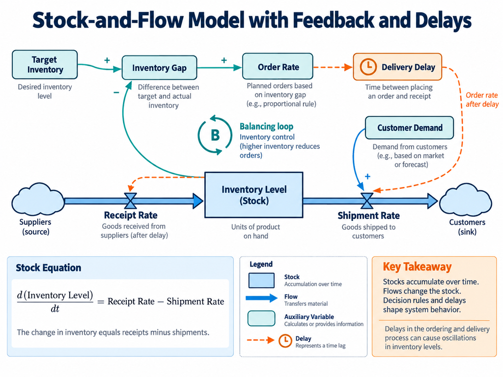
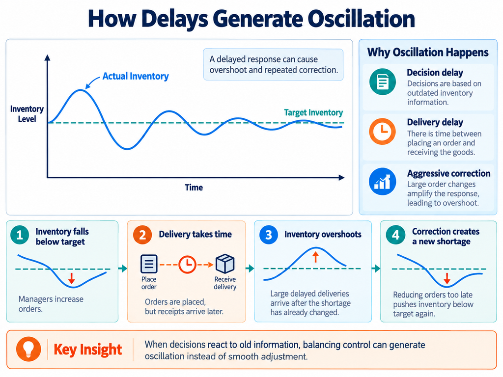
For example, inventory management involves interactions among customer demand, inventory levels, ordering decisions, and delivery lead times. When inventory becomes insufficient, purchase orders increase. However, deliveries take time. If additional orders are placed before earlier orders arrive, excess inventory may eventually accumulate.
Understanding this problem may require more than identifying the immediate cause of the inventory shortage. It may be necessary to investigate how ordering decisions, delivery delays, and inventory accumulation interact to generate behavior over time.
System Dynamics represents these structures using Stocks, Flows, variables, and equations. Models can then be simulated on a computer to examine how changes in assumptions, conditions, or policies may affect future behavior.
However, simulation results do not automatically establish that the causal relationships and parameters assumed in the model are correct. The results depend on how the real system has been represented.
The purpose of System Dynamics is not merely to calculate future numerical values. It is to understand how a system’s structure generates its behavior and examine how different interventions and decisions may change that behavior.
The History and Development of System Dynamics
System Dynamics was developed by Jay W. Forrester at MIT during the 1950s. Its initial focus was on examining business problems involving inventory, manufacturing, distribution, and order processing as dynamic systems with feedback.
Forrester’s 1961 book Industrial Dynamics systematically presented the methodology.
He subsequently published Urban Dynamics in 1969 and World Dynamics in 1971, extending the approach to urban and global problems.
The 1972 book The Limits to Growth used a world model incorporating interactions among population, resources, industrial production, food production, and pollution.
System Dynamics therefore developed during an era when computers were far less powerful than today’s machines.
Compared with modern AI and machine learning, it may consequently appear to be an old technology.
However, research and implementation have continued to advance. Recent developments in data analysis, statistical estimation, AI, and integration with other simulation methodologies have introduced new possibilities.
| Period | Major Developments |
|---|---|
| 1950s–1960s | Mathematical modeling of feedback and accumulation in business operations |
| 1970s–1980s | Applications to cities, environmental systems, economies, and social systems |
| 1990s–2000s | GUI-based model construction, organizational learning, and policy analysis |
| 2010s | Greater use of open model formats, Python integration, and multimethod simulation |
| 2020s | AI-assisted model construction, Bayesian estimation, hybrid modeling, and structural analysis of model behavior |
To understand these developments, it is important to distinguish the fundamental principles of System Dynamics from the technologies now being integrated with it.
Fundamental Principles of System Dynamics
In their 2024 paper “What Is (Quantitative) System Dynamics Modeling?”, published in System Dynamics Review, Asmeret Naugle, Saeed Langarudi, and Timothy Clancy identified five defining characteristics of quantitative System Dynamics.
| Fundamental Principle | Description |
|---|---|
| Causal Feedback Structure | The model is based on structures in which system components influence one another |
| Accumulation and Delays | Stocks and time delays are fundamental elements |
| Mathematical Representation | Relationships are represented using equations |
| Continuous-Time Perspective | The model represents states that change continuously over time |
| Feedback-Based Explanation | The analysis investigates how system structure generates behavior over time |
These characteristics help distinguish System Dynamics from other simulation methodologies.
For example, when the objective is to reproduce how individual products move through a manufacturing process, Discrete-Event Simulation may be appropriate.
When the objective is to represent the behavior of individual workers or customers, Agent-Based Modeling may be useful.
System Dynamics is particularly suited to examining overall changes driven by accumulation and feedback, often using relatively aggregated variables.
However, these methods can also be combined.
Modeling with Stocks and Flows
System Dynamics distinguishes between Stocks and Flows.
A Stock is a quantity that accumulates over time.
A Flow is a rate that increases or decreases a Stock.
For example, warehouse inventory is a Stock, while receipt and shipment rates are Flows.
Let (S(t)) represent inventory, (I(t)) the receipt rate, and (O(t)) the shipment rate.
A simplified model is:
[
\frac{dS(t)}{dt}=I(t)-O(t)
]
This equation states that the rate of change in inventory equals the receipt rate minus the shipment rate.
If inventory is measured in units, receipt and shipment rates may be measured in units per day.
However, this equation does not explain how the receipt and shipment rates are determined.
Additional relationships can therefore be introduced, including ordering policies, demand, delivery lead times, and supply capacity.
For example, an inventory shortage may increase the ordering rate, while increased ordering leads to greater receipts after a delay.
Combining such relationships transforms a simple accumulation equation into a dynamic model containing feedback.
Although System Dynamics adopts a continuous-time perspective, computers generally solve these models using numerical integration.
If the numerical time step is too large, the calculation may introduce artificial oscillations or numerical instability. Appropriate numerical methods and accuracy checks are therefore necessary.
Causal Loop Diagrams and Stock-and-Flow Models
System Dynamics uses both Causal Loop Diagrams (CLDs) and Stock-and-Flow Diagrams (SFDs).
A Causal Loop Diagram represents causal relationships among variables and visualizes Reinforcing and Balancing Feedback Loops.
A Stock-and-Flow Diagram explicitly identifies what accumulates and how inflows and outflows change those accumulated quantities.
| Perspective | Causal Loop Diagram | Stock-and-Flow Diagram |
|---|---|---|
| Main Purpose | Understand feedback structures | Model accumulation and change over time |
| Main Elements | Variables, causal links, feedback loops | Stocks, Flows, auxiliary variables, equations |
| Numerical Simulation | Usually cannot be performed from the diagram alone | Possible when equations and parameters are defined |
| Typical Applications | Problem structuring and causal hypothesis development | Dynamic simulation, policy comparison, sensitivity analysis |
Causal Loop Diagrams are useful for understanding the problem being modeled. However, a conventional CLD does not uniquely determine a valid Stock-and-Flow Model.
For example, an arrow indicating that advertising expenditure positively affects sales does not specify whether the relationship is linear, saturating, or delayed.
Converting that relationship into a mathematical model requires more precise definitions.
Bridging the gap between qualitative Causal Loop Diagrams and executable quantitative models has therefore become an important area of research.
Technological Advance 1 — Data-Driven Model Estimation
Early System Dynamics models frequently relied on expert knowledge and existing statistical information to define model structures and parameters.
However, simulation results may fail to reproduce real behavior if the parameters are inappropriate.
For example, the delay between increased recruitment and a larger effective workforce, or the relationship between inquiry volume and response time, may need to be estimated from observed data.
Modern statistical estimation and optimization methods can now be integrated more easily into System Dynamics workflows.
For example, model parameters can be adjusted to minimize the differences between an observed inventory time series and the inventory levels reproduced by the simulation.
However, fitting a model to observed data is not equivalent to establishing that its causal structure is correct.
Different model structures may reproduce similar time series.
Moreover, when several parameter combinations produce nearly identical results, estimating individual parameters uniquely may be difficult.
This is related to the problem of parameter identifiability.
Data-driven parameter estimation is an important advancement in connecting models with reality, but it does not eliminate the need to validate causal assumptions.
Technological Advance 2 — Bayesian Estimation and Uncertainty
Conventional parameter estimation often focuses on finding a single set of parameters that best fits observed data.
However, actual models may contain considerable uncertainty.
Observations may be insufficient, or multiple parameters may produce similar effects.
Bayesian estimation makes it possible to represent parameters through probability distributions rather than only point estimates.
This enables uncertainty to be incorporated explicitly into the analysis.
For example, rather than assuming a single fixed customer churn rate, a business model could use a distribution representing plausible churn rates based on available observations.
Repeated simulations using these distributions could then produce a range of possible outcomes for future customer numbers and revenue.
However, Bayesian results depend on assumptions about prior distributions, observation models, and model structures.
Bayesian inference itself is not a new technology. The recent development is the increasing feasibility of applying sophisticated inference methods to complex System Dynamics models.
Deep Learning for Parameter Estimation
In 2025, Hazhir Rahmandad, Ali Akhavan, Mohammad S. Jalali, and colleagues published “Incorporating Deep Learning Into System Dynamics: Amortized Bayesian Inference for Scalable Likelihood-Free Parameter Estimation” in System Dynamics Review.
The study applied Amortized Bayesian Inference (ABI) to System Dynamics.
ABI uses simulated data to train a neural network that can efficiently estimate posterior parameter distributions for new observations.
In this approach, a System Dynamics model generates simulated datasets, which are then used to train a machine-learning model for statistical inference.
The researchers examined the feasibility of the approach using two relatively simple System Dynamics models.
This represents more than an improvement in computational speed.
It combines simulation-based modeling with deep-learning-based statistical inference to estimate parameters while explicitly considering uncertainty.
However, the study does not establish that arbitrary large-scale System Dynamics models can already be estimated accurately through this approach.
Technological Advance 3 — Quantitative Analysis of Feedback Contributions
Causal Loop Diagrams can identify Reinforcing and Balancing Feedback Loops.
However, when multiple loops exist, the diagram alone cannot determine which loops contribute most strongly to the system’s observed behavior.
Research on Loop Dominance Analysis addresses this problem.
For example, consider a company’s user base that grows rapidly before its growth rate declines.
The model may contain a Reinforcing Loop in which existing users generate referrals and a Balancing Loop in which inadequate support capacity increases cancellations.
Simply identifying these two loops does not establish which one is primarily responsible for changes in the growth rate.
Loop Dominance Analysis uses the model’s structure and simulated behavior to investigate the contributions of different feedback loops.
In 2024, John Hayward and Paul A. Roach published “A Comparison of Loop Dominance Methods: Measures and Meaning,” comparing different methods and their interpretations.
An important challenge in this field is defining what it means for a loop to contribute to a particular behavior and presenting that information in a form that analysts can understand.
This research illustrates an important direction in the development of System Dynamics: moving beyond generating simulation results toward explaining why the model produces particular patterns of behavior.
However, such explanations refer to the internal structure of the model.
They do not automatically prove that the same causal structure exists in the real system.
Technological Advance 4 — Hybrid Simulation
System Dynamics is well suited to examining aggregate quantities and feedback.
However, real systems sometimes require detailed representations of individual entities or the order in which particular events occur.
For example, a manufacturing model that represents overall work-in-process inventory and production rates may not reproduce the precise sequence in which individual products pass through different machines.
This motivates combining different simulation methodologies.
| Method | Main Focus | Example Applications |
|---|---|---|
| System Dynamics (SD) | Accumulation, flows, feedback | Inventory, demand, investment, long-term organizational change |
| Discrete-Event Simulation (DES) | Individual events and processing sequences | Manufacturing operations, queues, equipment utilization |
| Agent-Based Modeling (ABM) | Individual agents and their interactions | Customer behavior, epidemics, competition among firms |
For example, a SaaS business could use System Dynamics to model the accumulation of customers and revenue while using an Agent-Based Model to represent purchasing or cancellation decisions among different customer segments.
A manufacturing system could use System Dynamics to examine long-term demand and investment while Discrete-Event Simulation represents the movement of individual products through equipment and production stages.
Hybrid Simulation combines models operating at different levels of abstraction.
In 2024, Le Khanh Ngan Nguyen, Susan Howick, and Itamar Megiddo published “A Framework for Conceptualising Hybrid System Dynamics and Agent-Based Simulation Models,” which examined conceptual model design for integrating SD and ABM.
Research reviews published in 2026 have also identified increasing interest in hybrid SD–ABM approaches while emphasizing continuing challenges involving validation, reproducibility, and interpretability.
Hybrid modeling is an important advancement, but combining multiple simulation methods is not always necessary or desirable.
Integration requires appropriate definitions of variable correspondences, time progression, and information exchange between models.
Technological Advance 5 — Integration with Python and Data Science
System Dynamics has traditionally been implemented through specialized modeling software.
Tools such as Vensim, Stella, and AnyLogic remain in use, but options are also available for working with models through programming environments such as Python.
One representative open-source project is PySD.
PySD is a Python library that supports working with System Dynamics models written in formats such as Vensim and XMILE.
It allows System Dynamics models to be combined with Python’s broader ecosystem of data analysis and machine-learning libraries.
Potential applications include:
- Estimating model parameters using observed data
- Running many simulations under different parameter settings
- Evaluating simulation results through statistical analysis
- Comparing interventions using optimization algorithms
- Approximating selected relationships using machine learning
Models and analytical functions can also be incorporated into larger software applications.
This represents a shift from treating System Dynamics as an activity confined to specialized software toward using it as a component of broader data analysis and simulation environments.
However, supported features and model formats differ among libraries.
The ability to execute a model in Python also does not establish that the model is valid.
Technological Advance 6 — Model Generation Using LLMs
One of the most significant recent developments is the use of Large Language Models to assist in model construction.
Traditionally, building a System Dynamics model required human modelers to identify variables, describe causal relationships, define Stocks and Flows, and construct equations.
This requires specialized knowledge and has been one of the barriers to wider adoption.
LLMs introduce the possibility of extracting model components from natural-language descriptions.
For example, consider the following statement:
“Customer inquiries are increasing, and the number of unresolved requests is growing. Hiring additional support staff improves processing capacity, but recruitment and training take time.”
An LLM could propose variables such as unresolved requests, inquiry arrival rate, resolution rate, and number of available support staff.
It could also suggest causal relationships and possible Stock-and-Flow structures.
2024 — Generating Causal Loop Diagrams from Text
In 2024, Niyousha Hosseinichimeh and colleagues published “From Text to Map: A System Dynamics Bot for Constructing Causal Loop Diagrams.”
The study proposed using LLMs to generate Causal Loop Diagrams from natural-language text.
The researchers evaluated the approach using 20 diagram-text pairs derived from System Dynamics literature, along with responses from 30 participants.
They reported that the system identified approximately 60% of the links and feedback loops in the evaluated material.
This result demonstrates the potential for automation while also showing that the approach did not completely reproduce the underlying structures.
2026 — Generating Executable Models
In 2026, William Schoenberg published “Building and Learning With Models Using AI” in System Dynamics Review.
The paper introduced an open-source framework called sd-ai.
It includes capabilities for generating Stock-and-Flow Models, equations, units, and documentation from natural-language inputs, as well as explaining simulation results through interactive dialogue.
The approach also explores the use of feedback-structure analysis to provide explanations of model behavior.
This represents an important development beyond asking an LLM merely to draw a Causal Loop Diagram.
The objective is to support the construction and analysis of executable mathematical models.
However, AI-generated models still require human validation and correction.
A model that executes successfully and contains syntactically valid equations is not necessarily an accurate representation of reality.
Technological Advance 7 — From Causal Loop Diagrams to Executable Models
Causal Loop Diagrams provide an accessible way to describe causal structures.
However, conventional CLDs generally lack some of the information needed to construct mathematical models.
For example, they may not identify whether a variable represents a Stock or a Flow.
Similarly, stating that one variable has a positive influence on another does not specify the mathematical relationship between them.
A 2026 study titled “Graph Notation as a Gateway—Transitioning from Causal Loop to Stock and Flow Diagrams (and Beyond) in System Dynamics Modeling” proposed an extended notation called CLD+.
CLD+ provides additional structural information beyond conventional Causal Loop Diagrams.
For example, it can distinguish Stocks from Flows, material flows from informational influences, and relationships involving significant delays.
Making these distinctions explicit can clarify the transition toward Stock-and-Flow representations.
However, this does not mean that every conventional Causal Loop Diagram can be automatically converted into a valid quantitative model.
Even when the model structure is defined, numerical simulation still requires suitable equations and parameters.
Nevertheless, this is an important research direction for connecting qualitative problem structuring with executable mathematical models.
Technological Advance 8 — The Relationship to Digital Twins
A Digital Twin connects a digital model with information about a real physical or operational system, supporting monitoring, analysis, prediction, optimization, or related functions.
Digital Twins are not synonymous with System Dynamics.
For example, modeling a machine’s temperature, vibration, or wear at high temporal resolution may require physical simulation or state estimation.
By contrast, System Dynamics may be appropriate for examining longer-term changes in factory investment, maintenance capacity, workforce levels, and inventory.
Another possibility is to update a model’s states or parameters using operational data, reducing the divergence between the model and the real system.
However, connecting a System Dynamics model to sensor data does not automatically create a reliable Digital Twin.
It is still necessary to determine how model states and parameters should be updated, how unobservable states should be handled, and what predictive accuracy can be achieved.
Research published in 2026 continues to identify synchronization between models and real-world data, together with rigorous validation in operational environments, as important challenges for Digital Twins.
Integration with Digital Twins is therefore one direction for expanding the applications of System Dynamics, but System Dynamics is not necessary for every Digital Twin.
What Has Changed in Modern System Dynamics?
The technological developments described above can be summarized by comparing traditional practices with newer approaches.
| Perspective | Traditional Approach | Recent Developments |
|---|---|---|
| Model Construction | Experts manually define variables and equations | LLM-assisted drafting of model structures and equations |
| Parameter Estimation | Expert judgment, optimization, established statistical methods | Bayesian estimation and deep-learning-assisted inference |
| Model Analysis | Comparison of simulation results | Structural contribution analysis, including Loop Dominance |
| Simulation Methods | Standalone System Dynamics models | Integration with ABM, DES, and other simulation approaches |
| Implementation Environment | Specialized software environments | Python, open model formats, external analytical libraries |
| Models and Data | Initial calibration and periodic updates | Potential integration with dynamic updates and data assimilation |
| User Interaction | Modelers interpret and explain results | AI-assisted interactive model construction and explanation |
However, these developments are at different stages of maturity.
Python-based model execution and hybrid simulation already have available implementations and practical applications.
By contrast, fully automated construction and validation of complex System Dynamics models using LLMs remains an area with substantial room for further research.
Modern tools do not automatically guarantee model validity.
Why System Dynamics Remains Useful
System Dynamics is an established methodology, but its fundamental concerns remain relevant.
Business and social problems often involve interacting factors whose consequences feed back into the processes that produced them.
Pricing, advertising, production capacity, inventory, R&D investment, and employee development may all influence one another over time.
An intervention may be effective in the short term while creating new constraints or problems in the longer term.
System Dynamics provides a framework for examining how relational structures can generate such behavior.
This purpose is different from simply improving predictive accuracy.
For example, a machine-learning model may forecast next month’s sales with high accuracy.
However, that predictive performance does not necessarily mean the model can correctly estimate what would happen if the company changed its prices or advertising expenditure.
Evaluating such interventions requires assumptions about causal relationships between actions and outcomes.
System Dynamics is one approach to representing these causal mechanisms explicitly.
However, the fact that a mathematical model includes causal arrows and equations does not establish that the assumed relationships are empirically correct.
Constructing a causal model and validating that model are separate tasks.
System Dynamics and Machine Learning
System Dynamics and Machine Learning both use models and data, but they often approach problems differently.
| Perspective | System Dynamics | General Predictive Machine Learning |
|---|---|---|
| Main Purpose | Explain system mechanisms and behavior over time | Learn predictive relationships from data |
| Model Structure | Explicit assumptions about causation and accumulation | Depends on the data and learning algorithm |
| Role of Data | Calibration, estimation, and model validation | Central to model training |
| Intervention Analysis | Can examine policies if the causal structure is appropriate | Ordinary predictive models do not guarantee valid intervention estimates |
| Main Limitation | Model structures and assumptions may be incorrect | Predictions may rely on correlations that are difficult to interpret causally |
Here, Machine Learning refers primarily to general-purpose predictive modeling.
Machine Learning also includes research on causal inference, dynamical system identification, control, and physics-informed learning.
Therefore, it would be misleading to treat System Dynamics and Machine Learning as fundamentally opposing approaches.
A potentially useful combination is to describe the system’s relational structure through System Dynamics while estimating selected equations or parameters using Machine Learning.
Practical Example — Modeling Customer Support Capacity
Consider a System Dynamics model of unresolved customer support requests.
The backlog is a Stock.
New inquiries are an Inflow, and completed resolutions are an Outflow.
The model might include the following variables.
| Variable | Description |
|---|---|
| Unresolved Requests | Number of support cases currently awaiting resolution |
| Inquiry Arrival Rate | New inquiries received per unit of time |
| Resolution Rate | Cases completed per unit of time |
| Available Support Staff | Number of employees capable of handling requests |
| Productivity per Employee | Cases processed per employee per unit of time |
| Recruitment and Training Delay | Time between deciding to hire and increasing effective support capacity |
The backlog changes according to:
[
\frac{dB(t)}{dt}=A(t)-C(t)
]
Here, (B(t)) is the number of unresolved requests, (A(t)) is the inquiry arrival rate, and (C(t)) is the resolution rate.
The resolution rate may be constrained by the number of available staff and their individual processing capacities.
In reality, the complexity of inquiries, working hours, software performance, and backlog conditions may also affect processing capacity.
Additional relationships can then be introduced.
For example, an increasing backlog may encourage recruitment, while recruitment and training delays prevent support capacity from increasing immediately.
Such a model can be used to compare potential interventions.
| Intervention | Question to Investigate |
|---|---|
| Hiring More Support Staff | How much could the backlog be reduced? |
| Shortening Training Time | Could the delay before capacity increases be reduced? |
| Automating Support Tasks | Could productivity per employee be improved? |
| Improving FAQ Resources | Could the arrival rate of inquiries be reduced? |
| Improving Inquiry Forms | Could the time needed to resolve cases be reduced? |
However, the estimated effects depend on the model structure and parameters.
For example, improving FAQ resources may have little effect if most inquiries are complex.
Automating support may increase processing capacity, but poor answer quality could generate additional inquiries.
Alternative relationships must therefore be considered when constructing the model.
Limitations of System Dynamics
System Dynamics continues to face important limitations.
First, defining the model structure can be difficult.
For example, corporate revenue may depend on pricing, advertising, product quality, competition, customer satisfaction, and other factors.
It is not automatically clear which variables should be included or how their relationships should be represented.
Second, parameter estimation can be difficult.
When observations are limited or several parameters produce similar effects, reliable estimation may not be possible.
Third, reproducing historical data does not guarantee accurate predictions of future policy outcomes.
New conditions may generate behavior or relationships not adequately represented by the original model.
Fourth, excessively broad models may become difficult to understand, estimate, and validate.
Fifth, problems involving heterogeneous individuals or discrete events may not be represented adequately using conventional aggregated System Dynamics models alone.
Sixth, presenting simulation results as precise numerical values may lead users to overestimate their reliability.
Mathematical precision and real-world validity are different things.
System Dynamics in ThinkNavi
ThinkNavi positions System Dynamics as a method for progressing from Systems Thinking and Causal Loop Diagrams toward quantitative model analysis.
Systems Thinking provides a conceptual understanding of interdependence, feedback, and dynamic behavior.
Causal Loop Diagrams organize hypotheses about causal relationships and feedback structures.
System Dynamics goes further by defining Stocks, Flows, equations, and parameters, enabling simulations of change over time.
These three topics therefore have distinct roles.
| Method | Main Role |
|---|---|
| Systems Thinking | Understand interdependence, feedback, and dynamic behavior |
| Causal Loop Diagrams | Visualize causal hypotheses and feedback structures |
| System Dynamics | Analyze dynamic behavior and potential intervention effects through mathematical models |
For ThinkNavi Free, one possible implementation would allow users to define Stocks and Flows manually and simulate simple accumulation models.
For example, users could examine changes in inventory, customer numbers, or unresolved support requests by specifying inflow and outflow rates.
Relationships between variables could then be added, including feedback and delays.
However, it may not be necessary to develop a fully general-purpose simulation environment from the beginning.
Even a limited system that allows users to understand basic Stock-and-Flow structures and compare behavior under different conditions could provide substantial educational value.
Potential LLM-Assisted Functions
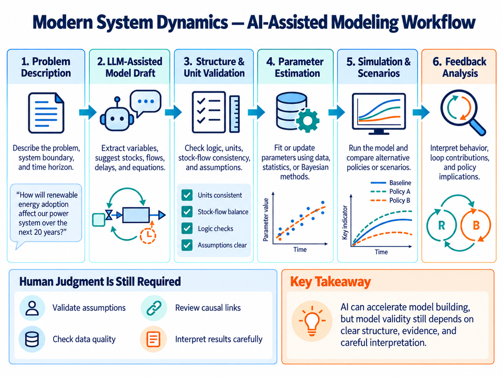
LLM-assisted functionality could begin with extracting variables and relational structures from natural-language problem descriptions.
Possible steps include:
- Extract variables from a problem description.
- Classify variables as Stocks, Flows, or auxiliary variables.
- Propose causal relationships and delays.
- Generate preliminary mathematical equations.
- Assist with parameter estimation and comparison against observed data.
- Explain simulation results and compare alternative interventions.
However, models generated by LLMs should not automatically be treated as correct.
Units, equation meanings, parameter sources, and initial conditions must be checked.
When causal conclusions are drawn from simulated intervention scenarios, the underlying causal assumptions must also be evaluated.
Is a Proprietary Simulation Engine Necessary?
The fundamental calculations used in System Dynamics involve the numerical solution of differential or difference equations.
Simple models can therefore be implemented using existing programming environments and numerical libraries.
For more sophisticated models, existing System Dynamics libraries such as PySD or integration with specialized software could be considered.
Developing a proprietary general-purpose engine would involve additional requirements, including numerical integration, delays, array variables, model consistency, and unit checking.
If ThinkNavi’s primary purpose is to help users understand and apply thinking methods, it may be more appropriate to begin with a limited set of reliable models rather than reproduce the full capabilities of specialized simulation software.
The Relationship to ConceptMiner
System Dynamics may also become relevant to knowledge exploration and analysis systems such as ConceptMiner.
For example, causal, control, and functional relationships could be extracted from technical documents and used to construct dynamic models of particular systems.
Comparing relational structures across different technological fields might also help identify candidate control mechanisms or supply-system designs.
However, discovering corresponding relational structures does not automatically provide an executable System Dynamics model.
Stocks and Flows must be identified, equations defined, units checked, and parameters estimated.
Furthermore, conceptual neighborhood relationships generated through Growing Neural Gas (GNG), relational mappings investigated through Structure-Mapping Theory, and causal dynamics modeled through System Dynamics represent different kinds of structures and processes.
Combining them might create a workflow linking information organization, cross-domain hypothesis generation, and dynamic model analysis.
However, the effectiveness of such a workflow would need to be demonstrated through concrete tasks and appropriate evaluation methods.
These are possibilities for future development and do not imply that all such capabilities are currently available.
Is System Dynamics an Outdated Technology?
System Dynamics certainly has a long history.
Its fundamental principles—Stocks, Flows, Feedback, and Delays—have also remained largely unchanged.
However, the age of these principles does not mean that the methodology has lost its value.
Recent developments include data-driven parameter estimation, Bayesian uncertainty analysis, integration with deep learning, hybrid simulation, quantitative feedback-structure analysis, and LLM-assisted model construction.
At the same time, the fundamental challenges of defining and validating model structures remain.
In particular, building a mathematical model containing causal relationships is different from demonstrating that those relationships accurately describe reality.
Furthermore, automating an established methodology through AI does not necessarily create a new scientific methodology.
Even when AI reduces the workload involved in model construction, expert judgment remains important for interpretation and validation.
The recent evolution of System Dynamics lies not in replacing its fundamental mathematical principles, but in making models easier to construct, estimate from data, analyze, validate, and integrate with other technologies.
Related Topics
- Systems Thinking — Understanding Interdependence, Feedback, and Change Over Time
- Causal Loop Diagrams — Visualizing Feedback Structures and Understanding System Behavior
- Logical Thinking — Building Sound Arguments, Communicating Reasoning, and Achieving Mutual Understanding
- Problem Structuring — Breaking Down Problems, Understanding Relationships, and Finding Paths to Solutions
- Root Cause Analysis (RCA) — Understanding Why Problems Occur and Preventing Recurrence
- KPI Trees — Decomposing Performance Goals and Identifying Levers for Improvement
- Concept Maps — Representing Relationships Between Concepts and Understanding Knowledge Structures
- Structure-Mapping Theory | Understanding Relational Correspondences and Generating New Inferences Across Domains
- Analogy — Connecting Knowledge Across Domains to Generate New Ideas and Hypotheses
- Design of Experiments (DOE) — Investigating Multiple Factors and Their Interactions Through Systematic Experimentation
- What Is Statistics? — Discovering Patterns in Data and Understanding an Uncertain World
- Multivariate Analysis — Discovering Relationships and Structures Among Multiple Variables
- Qualitative and Quantitative Thinking — Two Perspectives on Understanding the World and Their Integration
- gScenario Planning | Exploring Multiple Futures
- Critical Thinking | Examining Claims and Evidence
- The Scientific Method and Falsifiability — Generating Hypotheses and Testing Them Critically
- Concept Exploration | Discovering Emerging Concepts and Unknown Possibilities
References and Further Reading
Foundational Literature
- Jay W. Forrester, Industrial Dynamics, MIT Press, 1961.
- Jay W. Forrester, Urban Dynamics, MIT Press, 1969.
- Jay W. Forrester, World Dynamics, Wright-Allen Press, 1971.
- John D. Sterman, Business Dynamics: Systems Thinking and Modeling for a Complex World, Irwin/McGraw-Hill, 2000.
- Donella H. Meadows, Thinking in Systems: A Primer, Chelsea Green Publishing, 2008.
- Peter M. Senge, The Fifth Discipline: The Art & Practice of the Learning Organization, Doubleday, 1990.
Recent Research
- Asmeret Naugle, Saeed Langarudi, and Timothy Clancy, “What Is (Quantitative) System Dynamics Modeling? Defining Characteristics and the Opportunities They Create,” System Dynamics Review, 40(2), 2024.
- Hazhir Rahmandad, Ali Akhavan, and Mohammad S. Jalali, “Incorporating Deep Learning Into System Dynamics: Amortized Bayesian Inference for Scalable Likelihood-Free Parameter Estimation,” System Dynamics Review, 2025.
- John Hayward and Paul A. Roach, “A Comparison of Loop Dominance Methods: Measures and Meaning,” System Dynamics Review, 2024.
- Le Khanh Ngan Nguyen, Susan Howick, and Itamar Megiddo, “A Framework for Conceptualising Hybrid System Dynamics and Agent-Based Simulation Models,” European Journal of Operational Research, 315(3), 2024, pp. 1153–1166.
- Niyousha Hosseinichimeh et al., “From Text to Map: A System Dynamics Bot for Constructing Causal Loop Diagrams,” System Dynamics Review, 2024.
- William Schoenberg, “Building and Learning With Models Using AI,” System Dynamics Review, 42(1), 2026.
- William Schoenberg, “The Qualitative Engine: Creating and Evaluating an Iterative AI Modeling Tool,” System Dynamics Review, 42(2), 2026.
- “Graph Notation as a Gateway—Transitioning from Causal Loop to Stock and Flow Diagrams (and Beyond) in System Dynamics Modeling,” International Journal of Social Research Methodology, 2026.
- “Agent-Based Modeling and System Dynamics Integrated with AI and Analytical Methods: A Structured Review of Hybrid Approaches, Applications, and Future Directions for Decision Making in Complex Systems (2021–2026),” Systems, 14(8), 2026.