

Sensitivity Analysis is an analytical method used to examine how changes in input values, parameters, or underlying assumptions affect the results of a mathematical model. It is widely applied in decision analysis, business planning, investment evaluation, research and development, engineering design, simulation, statistical modeling, and many other fields.
When making decisions, we rely on various assumptions. For example, evaluating the profitability of a new business requires estimates of future market size, sales volume, selling prices, and manufacturing costs. However, these values are rarely known with certainty. If market demand turns out to be lower than expected or development costs increase, the profitability of the business may change significantly.
Similarly, when evaluating several R&D projects, decision-makers may assign weights to criteria such as technical feasibility, market potential, and strategic importance. A relatively small change in these weights may alter which project receives the highest overall evaluation.
Sensitivity Analysis addresses such problems by examining which input conditions have the greatest influence on results, how much those conditions must change before conclusions change, and how stable the current evaluation is under different assumptions.
The value of Sensitivity Analysis lies not merely in examining numerical results, but in understanding which assumptions those results depend on and evaluating the robustness of the resulting judgments.
Basic Principles of Sensitivity Analysis
A mathematical model can generally be expressed as a relationship between input variables and an output variable.
Y = f(X₁, X₂, …, Xₙ)
Here, X₁, X₂, …, Xₙ represent input variables or model parameters, while Y represents the calculated output.
Sensitivity Analysis examines how Y changes when one or more input variables are modified.
For example, suppose annual profit is calculated as follows:
Annual Profit = (Selling Price − Unit Variable Cost) × Sales Volume − Fixed Costs
This model contains four input variables: selling price, unit variable cost, sales volume, and fixed costs.
Changing the selling price may affect profit differently from changing sales volume. Furthermore, if reducing the selling price increases sales volume, the relationship between those two variables must also be considered.
Sensitivity Analysis helps identify which factors strongly influence profitability and which assumptions should receive priority in further investigation.
However, sensitivity refers to how a specified mathematical model responds to changes in its inputs. High sensitivity to a particular variable does not automatically establish that the variable is the most important cause of an outcome in the real world.
If the model omits important relationships, its sensitivity analysis may also produce misleading conclusions.
Example: Evaluating R&D Projects
Consider three R&D projects evaluated according to market potential, technical feasibility, and strategic importance.
| Project | Market Potential | Technical Feasibility | Strategic Importance |
|---|---|---|---|
| A | 8 | 6 | 7 |
| B | 6 | 9 | 8 |
| C | 9 | 5 | 6 |
Each criterion is evaluated on a scale from 0 to 10, with higher values representing more desirable characteristics. The values are hypothetical.
Suppose the weights assigned to the criteria are 40% for market potential, 35% for technical feasibility, and 25% for strategic importance.
The weighted overall scores are:
| Project | Overall Score | Rank |
|---|---|---|
| A | 7.05 | 2 |
| B | 7.55 | 1 |
| C | 6.85 | 3 |
Project B receives the highest score.
Now suppose the importance of market potential is increased to 60%, while the weight of technical feasibility is reduced to 15%. Strategic importance remains at 25%.
The results change as follows.
| Project | Original Weights | Modified Weights |
|---|---|---|
| A | 7.05 | 7.45 |
| B | 7.55 | 6.95 |
| C | 6.85 | 7.65 |
The highest-ranked project changes from B to C.
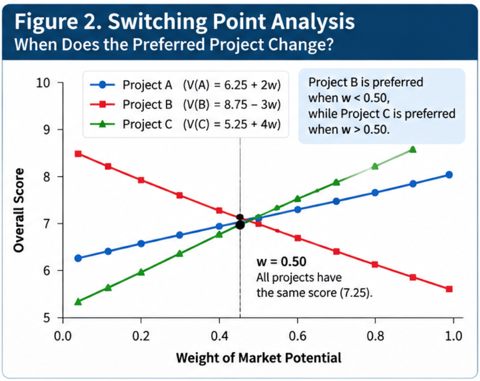
We can investigate this relationship further by changing the weight of market potential continuously.
Let w represent the weight of market potential. Keep the weight of strategic importance fixed at 0.25, and assign the remaining weight, 0.75 − w, to technical feasibility.
The overall scores can then be expressed as:
Project A: V(A) = 6.25 + 2w
Project B: V(B) = 8.75 − 3w
Project C: V(C) = 5.25 + 4w
When w equals 0.50, all three projects receive exactly the same score of 7.25.
Therefore, within this evaluation model, Project B ranks first when the market potential weight is below 50%, while Project C ranks first when it exceeds 50%.
This identifies the exact condition under which the preferred alternative changes.
The important insight is not simply that the rankings change. It is that we can identify the value judgments responsible for those rankings.
Whether market potential should receive a weight of 40% or 60% cannot be determined by mathematics alone. The appropriate weighting depends on business strategy, R&D objectives, investment horizons, and other organizational considerations.
Sensitivity Analysis provides information that helps decision-makers examine these judgments.
Local and Global Sensitivity Analysis
Sensitivity Analysis can broadly be divided into two categories: Local Sensitivity Analysis and Global Sensitivity Analysis.
Local Sensitivity Analysis examines how small changes in input variables affect model outputs near a particular reference point.
For example, it may estimate how much profit changes when the selling price increases by 1% from its current value.
Mathematically, local sensitivity can be expressed using a partial derivative.
Sᵢ = ∂Y / ∂Xᵢ
However, comparing derivatives directly may be inappropriate when input variables have different units. Dimensionless or normalized sensitivity coefficients are often used to make the results more comparable.
Global Sensitivity Analysis, by contrast, considers the behavior of the model across broader ranges of input values.
For example, selling prices, market demand, and manufacturing costs may each vary within specified ranges. Global methods examine the model under many combinations of these inputs.
This makes it possible to investigate nonlinear relationships and interactions among variables that may be overlooked by local analysis.
| Aspect | Local Sensitivity Analysis | Global Sensitivity Analysis |
|---|---|---|
| Scope | Near a reference point | Across broader input ranges |
| Typical methods | Derivatives, finite differences | Morris, Sobol, FAST |
| Computational cost | Usually relatively low | Often higher |
| Nonlinear behavior | Examines effects near a point | Can explore effects across the input space |
| Interactions | Limited in simple one-factor analyses | Can be evaluated by appropriate methods |
| Typical applications | Preliminary analysis, simple models | Complex simulations, model validation |
The distinction concerns the scope and interpretation of the analysis. One-factor perturbation methods can also be applied at multiple points across an input space, as in the Morris method.
One-at-a-Time (OAT) Analysis
One of the simplest forms of Sensitivity Analysis is One-at-a-Time (OAT) analysis.
In this approach, one input variable is changed while the others are held constant.
For example, in a business profitability model, an analyst might separately increase and decrease selling price, sales volume, and manufacturing costs by 10%, then calculate the corresponding changes in profit.
This approach is easy to understand and requires relatively little computation, making it useful for preliminary analysis.
However, it has important limitations.
If changing the selling price also changes sales volume, treating the two variables as completely independent may not represent the actual business situation.
Similarly, when the effect of one variable depends on the value of another, changing each variable separately around a single reference point may fail to reveal the interaction.
OAT analysis is therefore a useful starting point, but it cannot address every sensitivity analysis problem.
Tornado Charts
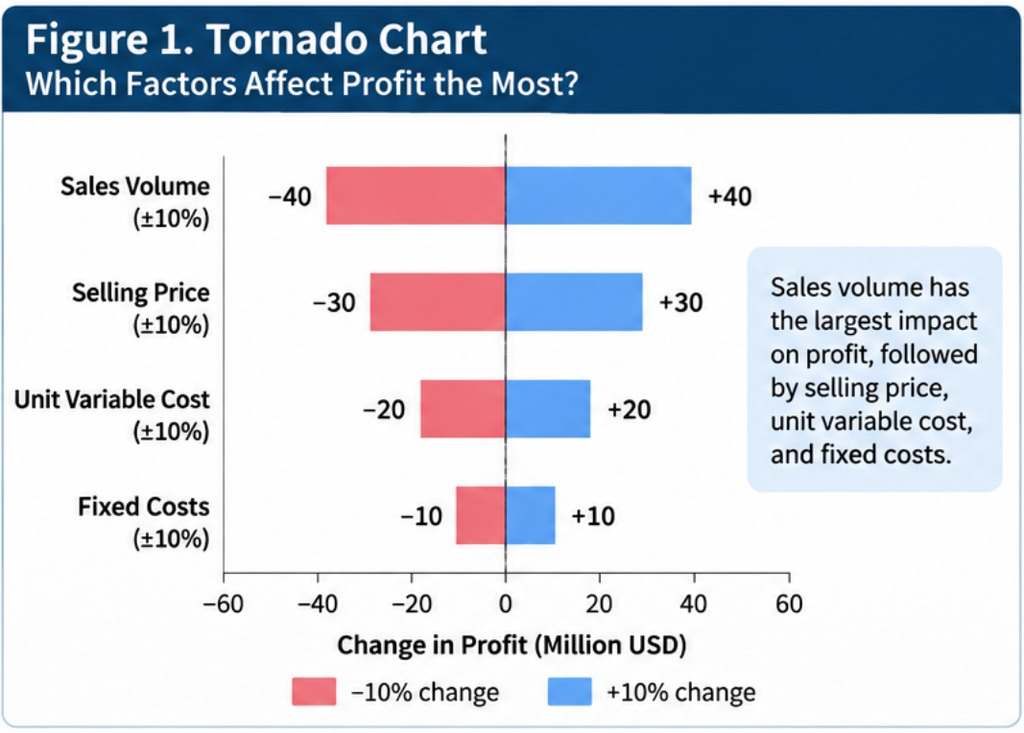
A Tornado Chart is one of the most common ways to visualize the results of Sensitivity Analysis.
It uses horizontal bars to represent how much the model output changes when individual input variables are varied over specified ranges.
The variables are usually ordered according to the magnitude of their effects, producing a shape resembling a tornado.
For example, when evaluating the profitability of an equipment investment, a Tornado Chart may compare the effects of changes in sales volume, manufacturing costs, selling prices, and maintenance expenses.
This allows users to identify which assumptions have the largest influence on the calculated return.
However, the length of each bar also depends on the range assigned to the corresponding input variable.
If sales volume is varied by ±30% while manufacturing costs are varied by only ±5%, sales volume may appear much more influential simply because a larger range was examined.
Therefore, the input ranges used in a Tornado Chart should always be reported alongside the results.
Sensitivity Analysis with Interactions
When a model contains multiple input variables, their effects may not be independent.
For example, consider an R&D project’s business value as a function of technical feasibility and market growth.
If market growth is low, even a technically feasible project may generate limited business value. Conversely, when market growth is high, improving technical feasibility may create substantial additional value.
Such relationships can be represented through interaction terms, as in regression analysis.
Y = β₀ + β₁X₁ + β₂X₂ + β₃X₁X₂
Here, β₃X₁X₂ is the interaction term.
When this term is present, the effect of X₁ on Y depends on the value of X₂.
Sensitivity Analysis can examine such relationships by changing two or more variables simultaneously.
For example, two input variables can be assigned to the horizontal and vertical axes of a graph, while the calculated output is represented through contours or colors.
This produces a contour plot or heatmap showing which combinations of input conditions generate higher or lower results.
However, as the number of input variables increases, evaluating every possible combination becomes impractical.
This is where Design of Experiments (DOE) and Global Sensitivity Analysis become particularly valuable.
The Morris Method: Screening Important Variables
The Morris Method, also known as the Method of Morris, is a Global Sensitivity Analysis technique designed to identify influential variables in models with many inputs.
It evaluates changes in individual variables at multiple locations in the input space.
For each variable, it calculates quantities called Elementary Effects, which measure how changes in that variable affect the model output.
Two commonly used summary statistics are the absolute mean of the Elementary Effects, μ*, and their standard deviation.
A large μ* suggests that a variable may have a strong overall influence on the output.
A large standard deviation suggests that the variable’s effect changes substantially across the input space. This may indicate nonlinear behavior, interactions with other variables, or both.
The Morris Method does not provide a complete decomposition of all interactions. However, it can identify important variables with relatively few model evaluations.
It is therefore particularly useful as an initial screening method for complex simulation models.
The Sobol Method: Decomposing Output Variance
The Sobol Method is one of the most widely studied approaches to Global Sensitivity Analysis.
It decomposes the variance of a model’s output into contributions associated with individual input variables and their interactions.
Consider a business profit model with uncertain sales volume, selling prices, manufacturing costs, and fixed expenses.
By repeatedly evaluating the model under different combinations of input values, the Sobol Method can estimate how much each variable contributes to the overall variability of profit.
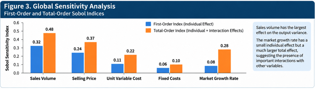
Two important measures are the First-Order Sensitivity Index and the Total-Order Sensitivity Index.
The First-Order Sensitivity Index measures the proportion of output variance attributable to the individual effect of a particular input variable.
The Total-Order Sensitivity Index includes both the individual effect of that variable and its interactions with other variables.
For example, a variable may have a small first-order index but a large total-order index. This suggests that the variable contributes substantially to output variability through interactions with other inputs.
The conventional Sobol variance decomposition assumes that the input variables are statistically independent. When inputs are correlated, alternative formulations or methods capable of handling dependencies are required.
Furthermore, Sobol indices depend on the specified input ranges and probability distributions.
They should not be interpreted as universal measures of the inherent importance of variables, independent of the assumptions used in the analysis.
Sensitivity Analysis and Monte Carlo Simulation
Monte Carlo Simulation uses repeated random sampling to calculate model outputs under uncertain input conditions.
For example, when forecasting the revenue or profitability of a new business, probability distributions may be assigned to market growth, selling prices, sales volume, and other variables.
The model is then evaluated thousands or tens of thousands of times using different sampled inputs.
The resulting output distribution can provide estimates of expected profit, variability, and the probability of operating at a loss.
However, Monte Carlo Simulation alone does not necessarily reveal which input variables are responsible for the uncertainty in the results.
Sensitivity Analysis can be applied to investigate those contributions.
For example, variance-based techniques such as the Sobol Method can be combined with appropriate sampling procedures to estimate the contributions of individual variables and interactions.
An important distinction should be made between two related concepts.
Uncertainty Analysis examines how uncertain the model output is, while Sensitivity Analysis investigates how changes in inputs contribute to changes or variability in that output.
The two approaches are closely related but address different questions.
Sensitivity Analysis and Robustness Analysis
Sensitivity Analysis is closely related to Robustness Analysis.
Sensitivity Analysis examines how outputs respond to changes in model inputs. Robustness Analysis focuses on whether a particular conclusion or decision remains valid under different assumptions or conditions.
For example, suppose R&D Project A remains the highest-ranked alternative even when the evaluation weights are varied across a reasonable range.
The decision may then be considered robust with respect to those weighting assumptions.
Conversely, if a small change in weights causes the preferred project to change, the decision may be sensitive or unstable.
However, high sensitivity is not necessarily undesirable.
If an important strategic judgment strongly influences the outcome, identifying that influence can itself be valuable.
Similarly, low sensitivity does not guarantee that the model is appropriate. A model may appear stable simply because it omits important factors or relationships.
Robustness should therefore be evaluated in relation to the conclusions that matter for the decision, rather than merely the numerical stability of the model output.
Sensitivity Analysis in Bayesian Networks
Sensitivity Analysis is also important in Bayesian Networks.
A Bayesian Network represents probabilistic dependencies among variables using a directed graph and Conditional Probability Tables (CPTs).
When CPT values are estimated from expert knowledge rather than extensive statistical data, considerable uncertainty may remain.
For example, an equipment failure model might assign a 60% probability of failure under excessive load.
However, the expert may believe that the appropriate value lies somewhere between 50% and 70%.
Sensitivity Analysis can examine how changes within this range affect posterior probabilities and diagnostic conclusions.
If the diagnosis remains almost unchanged across the plausible range, obtaining a more precise estimate of that CPT parameter may be relatively unimportant.
Conversely, if a small change produces a substantial shift in the diagnosis, the parameter may deserve closer examination.
When modifying CPT values, it is essential to maintain the requirement that the probabilities of all states under each parent-state configuration sum to 1.
Furthermore, a parameter’s sensitivity does not necessarily equal the economic value of obtaining additional information about it.
The Value of Information also depends on how the information affects possible decisions, expected consequences, and the cost of obtaining the information.
Sensitivity Analysis in R&D and New Business Development
Sensitivity Analysis is especially valuable in research and development and new business planning because these activities involve substantial uncertainty.
When evaluating R&D projects, decision-makers may consider technical feasibility, market potential, novelty, development costs, and strategic importance.
However, the more innovative a research project is, the more difficult it may be to estimate these characteristics reliably.
Sensitivity Analysis can help identify which evaluation criteria most strongly influence project rankings, which uncertain assumptions deserve additional investigation, and under what conditions project priorities change.
When several R&D projects are combined into an investment portfolio, sensitivity analysis can also investigate how changes in budgets, personnel allocation, or project interactions affect portfolio-level outcomes.
In new business development, it is often more important to identify the conditions under which a business becomes viable than simply to calculate whether it currently appears attractive.
For example, an analysis may reveal that an investment becomes profitable only when market demand exceeds a certain threshold, or that commercialization requires manufacturing costs to fall below a particular level.
Identifying the input value at which a decision or conclusion changes is often called Switching Value Analysis.
This approach shifts the question from:
“Is this business opportunity attractive?”
to:
“Under what conditions would this business opportunity become attractive?”
Sensitivity Analysis can therefore help transform a general evaluation into a more concrete investigation of the conditions required for success.
Limitations and Important Considerations
Several limitations must be considered when applying Sensitivity Analysis.
First, the results depend on the structure of the underlying model.
If the model does not represent important real-world relationships, even sophisticated sensitivity analysis may provide misleading guidance.
Second, the selection of input ranges can strongly influence the results.
Comparing one variable over a ±5% range with another over a ±50% range does not provide a neutral comparison of their intrinsic importance.
Third, dependencies among input variables must be considered.
Selling prices and sales volume, or technical feasibility and development costs, may be related. Varying them independently can produce combinations of assumptions that would be unlikely or impossible in practice.
Fourth, low sensitivity near a reference point does not imply low sensitivity everywhere.
In nonlinear models or models containing thresholds, a variable may have little effect under one set of conditions but a substantial effect elsewhere.
Fifth, sensitivity analysis should not be confused with proof of causality.
Changing a variable in a mathematical model is not necessarily equivalent to intervening on that variable in the real world.
Finally, Sensitivity Analysis cannot automatically discover important factors that have been omitted from the model.
Identifying unknown influences requires additional problem structuring, investigation, and critical examination of the model itself.
Sensitivity Analysis in the Age of AI
The development of Large Language Models (LLMs) creates new opportunities to make Sensitivity Analysis more accessible.
Traditionally, performing Sensitivity Analysis required users to understand the mathematical model, identify relevant input variables, specify plausible ranges, and execute the necessary calculations.
LLMs can assist with these preparatory activities through natural language interaction.
For example, a user might enter:
“I want to identify the major uncertainties affecting the profitability of a new business.”
An LLM could suggest potential variables such as market demand, selling prices, customer acquisition costs, manufacturing expenses, and development time.
It could also help retrieve market research, technical reports, or historical data relevant to estimating plausible input ranges.
However, the numerical ranges and probability distributions proposed by an LLM should not automatically be regarded as reliable.
Users must examine the evidence and determine whether the assumptions are appropriate for their particular situation.
The calculations themselves are better performed by a dedicated mathematical engine, while the LLM assists with variable selection, method selection, interpretation, and identifying questions for further investigation.
Another promising application is using Sensitivity Analysis to critically examine evaluation models generated or assisted by LLMs.
For example, if an LLM recommends a particular R&D project based on several evaluation criteria, Sensitivity Analysis can determine whether the recommendation remains stable when weights or scores are modified.
If the analysis identifies a particularly influential uncertainty, the user can ask the LLM to investigate that uncertainty further.
This creates an iterative process:
Model construction → Sensitivity analysis → Identification of critical assumptions → Additional research → Model revision
Such an approach combines the flexibility of LLM-assisted investigation with the mathematical transparency of structured analysis.
Sensitivity Analysis in ThinkNavi
ThinkNavi regards Sensitivity Analysis as a fundamental thinking-support method for examining the validity and stability of results produced by mathematical models.
ThinkNavi Free is planned to provide tools that allow users to modify input values and evaluation weights manually and visually examine how the results change.
In Decision Matrices and AHP, Sensitivity Analysis can be used to investigate changes in overall scores, changes in rankings, switching points, and the stability of evaluation results.
In Bayesian Networks, users could modify Conditional Probability Table values and examine the resulting changes in posterior probabilities.
In the future, these capabilities could be developed into a common Sensitivity Analysis framework applicable to different mathematical models.
Depending on the type of model and computational requirements, the framework could support OAT analysis, Tornado Charts, Monte Carlo Simulation, the Morris Method, and Sobol analysis.
Computationally demanding methods could be implemented through a shared mathematical analysis engine within the ConceptMiner product family.
In an LLM-assisted version, AI could help users identify relevant variables, propose plausible ranges, interpret results, retrieve information about important uncertainties, and critically examine the assumptions underlying the model.
Sensitivity Analysis could also be integrated into ConceptMiner R&D to evaluate hypotheses and research themes generated through concept exploration.
For example, users could examine the conditions under which a particular R&D theme becomes attractive and determine how robust that evaluation remains under alternative assumptions.
Sensitivity Analysis is not merely a technique for repeating calculations under different conditions.
It is a method for moving beyond the acceptance of a single numerical result and understanding the assumptions that make the result possible.
The essential question is not simply how much the result changes, but which assumptions can change the conclusion—and how strongly those assumptions are supported by evidence.
Sensitivity Analysis connects mathematical modeling with critical human thinking. It will continue to play an important role in decision support as computers and AI become increasingly involved in analytical processes.
Related Thinking Methods:
- Multi-Criteria Decision Analysis (MCDA) | Mathematical Approaches to Integrating Multiple Criteria and Value Judgments
- Decision Matrix | Comparing Alternatives Across Multiple Criteria and Evaluating Decision Validity
- , Analytic Hierarchy Process (AHP) | Quantifying Evaluation Criteria Through Pairwise Comparisons
- Analytic Network Process (ANP) | Decision-Making with Interdependencies and Feedback
- Bayesian Networks | Structuring Uncertainty and Reasoning with Probabilistic Models
- Scenario Analysis,
- Design of Experiments (DOE) — Investigating Multiple Factors and Their Interactions Through Systematic Experimentation
- Monte Carlo Simulation,
- Robustness Analysis,
- System Dynamics — Modeling Feedback Mathematically to Understand How Systems Change Over Time
References and Further Reading
- Andrea Saltelli, Marco Ratto, Terry Andres, Francesca Campolongo, Jessica Cariboni, Debora Gatelli, Michaela Saisana, and Stefano Tarantola, Global Sensitivity Analysis: The Primer, Wiley, 2008.
- Max D. Morris, “Factorial Sampling Plans for Preliminary Computational Experiments,” Technometrics, 33(2), pp. 161–174, 1991.
- Ilya M. Sobol’, “Global Sensitivity Indices for Nonlinear Mathematical Models and Their Monte Carlo Estimates,” Mathematics and Computers in Simulation, 55(1–3), pp. 271–280, 2001.
- Andrea Saltelli et al., “Variance Based Sensitivity Analysis of Model Output: Design and Estimator for the Total Sensitivity Index,” Computer Physics Communications, 181(2), pp. 259–270, 2010.
- European Commission Joint Research Centre — Sensitivity Analysis (SAMO)
- European Commission Joint Research Centre — Sensitivity Analysis Methods
- SALib — Sensitivity Analysis Library in Python
- UK Government — The Green Book (2026)